Polynomial interpolation does not always converge to the interpolated function with increasing number of points. In fact, it can be shown with methods of functional analysis, that for any scheme of interpolation points
![]()
there is a continuous function such that the interpolation does not converge.
Runge gave a counterexample for equi-spaced points.
>function f(x) &= 1/(1+5*x^2)
                                  1
                               --------
                                  2
                               5 x  + 1
We interpolate
![]()
in points
![]()
We use Newton's divided differences.
>xp=linspace(-1,1,40); yp=f(xp); dd=divdif(xp,yp);
Now, we plot
into one plot.
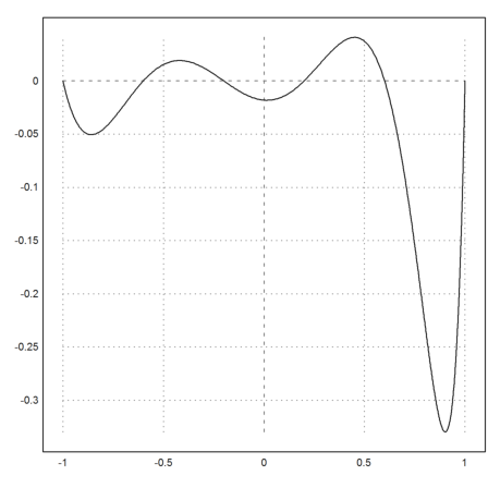
>plot2d("f(x)",color=blue,r=1); ...
 plot2d(xp,yp,points=true,style="+",add=true,color=red); ...
 plot2d("interpval(xp,dd,x)",add=true):
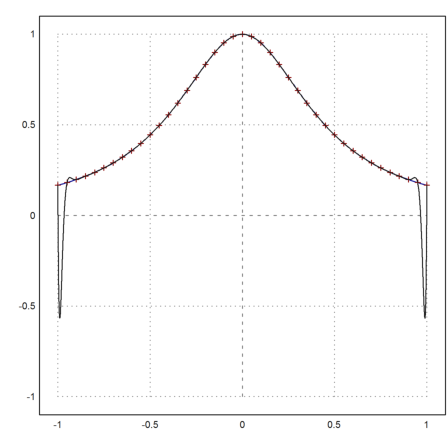
It becomes clear that something weird happens towards the ends of the interval.
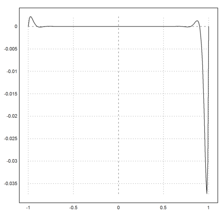
Here is the error function.
>plot2d("f(x)-interpval(xp,dd,x)",-1,1):
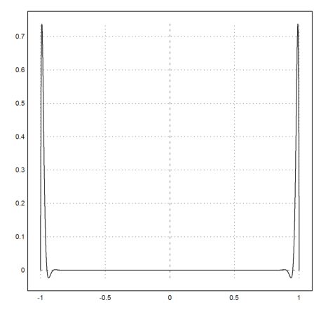
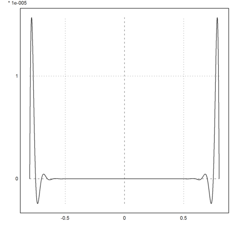
The error is quite small in the interior part of the interval.
>plot2d("f(x)-interpval(xp,dd,x)",-0.8,0.8):
To understand this, we need to consider a special interpolation formula.
We assume, we have interpolation points
![]()
>xp=linspace(-1,1,5); // thus n=5
Then we define a function
![]()
>function map om(x) := prod(x-xp)
Now we claim that
![]()
is the interpolating polynomial of degree n to the function
![]()
In fact, p interpolations in the zeros of omega, and it is a polynomial of degree n.
>function p(x) := (1-om(x)/om(a))/(a-x)
Let us test this by interpolating
![]()
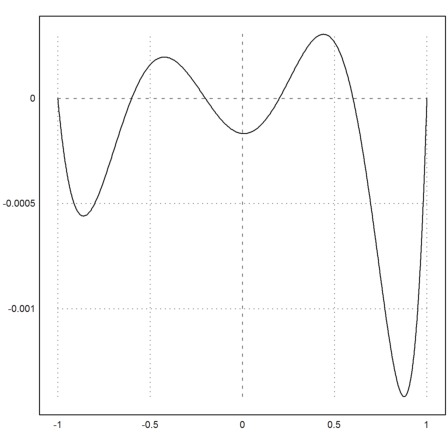
in 6 equispaced points. We plot the error function.
>a=2; plot2d("1/(a-x)-p(x)",-1,1):
The error gets larger, if we push the point a closer to the interval.
>a=1.2; plot2d("1/(a-x)-p(x)",-1,1):
With a little computation, we see
![]()
>function R(x) := om(x)/((a-x)*om(a))
>a=1.1; xp=linspace(-1,1,20); plot2d("R(x)",-1,1):
Let us compute the error in the last interval.
>R(fmin("R(x)",xp[-2],xp[-1]))
-0.0373216835811
What has this to do with Runge's example?
In fact, we can write the Runge function as the difference of two function of the type we just studied, scaled by a constant.
>&1/(x-I/a)-1/(x+I/a), &ratsimp(%)
                              1       1
                            ----- - -----
                                I       I
                            x - -   x + -
                                a       a


                                2 I a
                              ---------
                               2  2
                              a  x  + 1
Thus we can simply subtract the two interpolations. It turns out that one is minus the conjugate of the other, so we can simply study the convergence behavior of the interpolation of
![]()
Thus the convergence depends solely on the behavior of
![]()
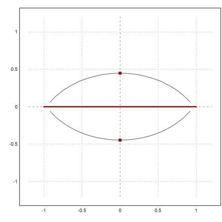
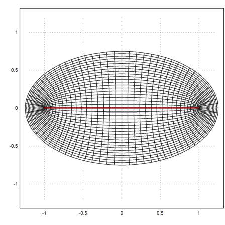
for n to infinity. We plot the omega in the complex plane, and include the interval [-1,1], where x is, and the point
![]()
Since omega grows very fast, we take the logarithm.
>plot2d("log(abs(om(x+I*y)))",r=1.2,>contour,levels="thin"); ...
 plot2d([-1,1],[0,0],thickness=3,color=red,add=true); ...
 plot2d([0,0],[-1/sqrt(5),1/sqrt(5)],color=red,points=true,style="[]#",>add):
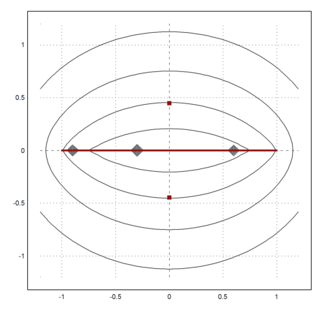
If we inspect this image closely, we see that the level lines of log(|omega|) through the points a end inside the interval [-1,1].
To study the behavior for n to infinity, we observe that
![]()
We can compute this integral exactly. The result is a long expression.
>function G(a,b) &= integrate(log((x-a)^2+b^2)/2,x,-1,1)|ratsimp
              ! 2    2          !                ! 2    2          !
       (a log(!b  + a  + 2 a + 1!) + (1 - a) log(!b  + a  - 2 a + 1!)
        2    2                      a + 1           a - 1
 + log(b  + a  + 2 a + 1) + (2 atan(-----) - 2 atan(-----)) b
                                      b               b
               2    2
 + I atan2(0, b  + a  - 2 a + 1) - 4)/2
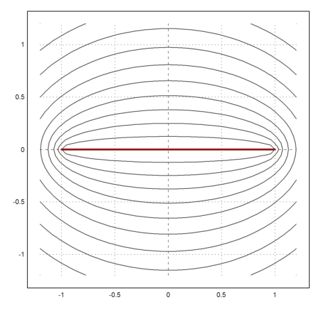
Let us plot this in the same way as above.
>plot2d("re(G(x,y))",r=1.2,>contour,levels="thin"); ...
 plot2d([-1,1],[0,0],thickness=3,color=red,add=true); ...
 plot2d([0,0],[-1/sqrt(5),1/sqrt(5)],color=red,points=true,style="[]#",>add):
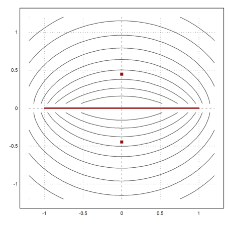
Here is an image with the level line through a only.
>plot2d("re(G(x,y))",r=1.2,level=re(G(0,1/sqrt(5)))); ...
 plot2d([-1,1],[0,0],thickness=3,color=red,add=true); ...
 plot2d([0,0],[-1/sqrt(5),1/sqrt(5)],color=red,points=true,style="[]#",>add):
Again, the level line through a passes through the interval [-1,1]. We can compute
![]()
Our function does not work for 1. We have to stay a little bit off the real line.
>exp(G(1,0.0001)) / exp(G(0,1/sqrt(5)))
1.19161+0i
The result is that the maximal error grows like
![]()
It will grow exponentially to infinity.
If we think about it, we see that the evenly spaced points are not optimal. It would be better, if omega was much larger in a than in [-1,1]. The solution is to use the zeros of the Chebyshev polynomials.
>xp=chebzeros(-1,1,20); yp=f(xp); dd=divdif(xp,yp); ...
 plot2d("f(x)",color=blue,r=1); ...
 plot2d(xp,yp,points=true,style="+",add=true,color=red); ...
 plot2d("interpval(xp,dd,x)",>add):
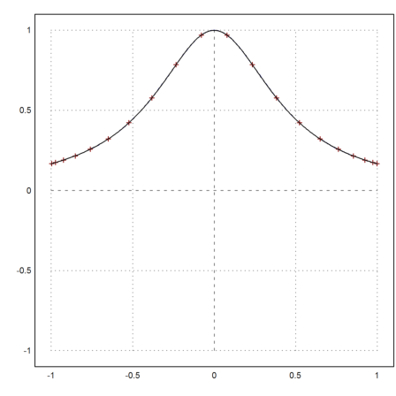
We see thant the approximation looks really good. this is confirmed, if we look at the error.
>plot2d("f(x)-interpval(xp,dd,x)",-1,1):
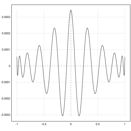
The error is about 0.0003.
In fact, the level line of omega now goes around the interval [-1,1].
>plot2d("log(abs(om(x+I*y)))",r=1.2,contour=true,levels="thin"); ...
 plot2d([-1,1],[0,0],thickness=3,color=red,add=true); ...
 plot2d([0,0],[-1/sqrt(5),1/sqrt(5)],color=red,points=true,style="[]#",>add):
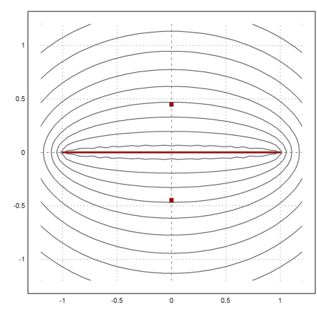
The limit distribution is called the Green's function of [-1,1].
![]()
with G(z)=0 if z converges to [-1,1]. G(z) is somewhat complicated to compute. We define the Joukowski mapping
![]()
which maps the outside of the unit circle to the outside of [-1,1].
>function J(w) &= (w+1/w)/2;
If we plot this, we see the level lines of G.
>r=linspace(1,2,20); phi=linspace(0,2pi,80)'; w=r*exp(phi*I); ...
 plot2d(J(w),r=1.2);  ...
   plot2d([-1,1],[0,0],color=red,add=true,thickness=3):
We have
![]()
We can make this a function, at least for the right half plane. For this we take the correct solution of w=G(z).
>&solve(J(w)=z,w), function G(z) &= log(abs(w with %[2])); $'G(z)=G(z)
                            2                 2
             [w = z - sqrt(z  - 1), w = sqrt(z  - 1) + z]
![]()
The problem with this approach is that the function takes the wrong branch of the square root function for re(x)<0.
>plot3d("G(x+I*y)",r=1.2,angle=220°):
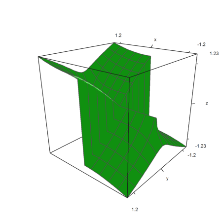
We fix it by observing that G must be symmetric to the imaginary axis.
>function Gt(z) := G(abs(re(z))+I*im(z))
>plot2d("Gt(x+I*y)",r=1.2,levels="thin");  ...
   plot2d([-1,1],[0,0],color=red,thickness=3,>add):
Indeed, for 50 points our omega is very close to G.
>xp=chebzeros(-1,1,50); ...
 log(om(1.5))/50+log(2)
0.962423650119
>G(1.5)
0.962423650119
Our error of approximation decreases exponentially with the following gamma.
>gamma=1/exp(G(I/sqrt(5)))
0.64823151951
For n=20, we expect the following order of magnitude.
>gamma^20
0.000171633826724